Clasificación de hojas sanas y enfermas
Entrenamiento de una CNN en PyTorch para detectar enfermedades en hojas de plantas. Pipeline completo: preprocesado de imágenes (6000×4000 → 224×224), data augmentation, entrenamiento y evaluación.
Clasificación de hojas: sanas o enfermas usando una CNN en PyTorch
En este notebook vamos a entrenar una CNN para clasificar imágenes de hojas en dos categorías: sanas o enfermas.
Más info sobre el dataset y cómo descargarlo:
https://www.tensorflow.org/datasets/catalog/plant_leaves?hl=es
Preprocesado de las imágenes
Las imágenes originales miden 6000x4000. Queremos primero recortar las imágenes para eliminar 1000 píxeles a la izquierda y 1000 a la derecha, quedando una imagen cuadrada de 4000x4000. Luego las redimensionamos a 224x224.
Guardaremos estas imágenes con el sufijo "_resized" en el mismo directorio. Si la imagen "_resized.JPG" ya existe, no haremos el procesamiento de nuevo.
Esta celda se debe ejecutar antes de la carga de datos, de forma que cuando creemos los dataloaders, ya carguemos sólo las imágenes redimensionadas.
import os
import glob
from PIL import Image

def preprocess_images(root, out=None):
    # Navegamos por todas las subcarpetas (plantas / healthy / diseased)
    for plant_dir in os.listdir(root):
        plant_path = os.path.join(root, plant_dir)
        if os.path.isdir(plant_path):
            # Buscamos en las carpetas healthy y diseased
            for condition in ["healthy", "diseased"]:
                condition_path = os.path.join(plant_path, condition)
                if os.path.isdir(condition_path):
                    # Procesamos todas las imágenes .JPG
                    for img_file in glob.glob(os.path.join(condition_path, "*.JPG")):
                        # Comprobar si ya existe la versión redimensionada
                        if "_resized" in img_file:
                            continue
                        basedir, filename = os.path.split(img_file)
                        name, ext = os.path.splitext(filename)
                        if out is None:
                            out = basedir
                        resized_dir = os.path.join(out, plant_dir, condition)
                        if not os.path.exists(resized_dir):
                            os.makedirs(resized_dir)
                        resized_file = os.path.join(resized_dir, name + "_resized" + ext)
                        if os.path.exists(resized_file):
                            # Si ya existe, saltamos
                            continue

                        # Abrimos la imagen original
                        print('Opening:', img_file)
                        with Image.open(img_file) as img:
                            # Verificamos el tamaño (debe ser 6000x4000)
                            w, h = img.size
                            # Recortamos 1000px de izq y der:
                            # Queremos un recorte centrado:
                            # Si el ancho es 6000, para llegar a 4000, quitamos 1000 a la izq y 1000 a la der.
                            left = 1000
                            upper = 0
                            right = w - 1000
                            lower = h  # altura permanece igual (4000)
                            cropped = img.crop((left, upper, right, lower))

                            # Redimensionamos a 224x224
                            resized = cropped.resize((224,224), Image.BILINEAR)

                            # Guardamos con "_resized"
                            resized.save(resized_file, "JPEG")

# Ejecutamos la función de preprocesado sobre el dataset
root_path = r"E:/temp/leafs/leafs"
out = r"E:/temp/leafs/resized/"
preprocess_images(root_path, out)
1. Generar la función para cargar el dataset con dataloaders
Vamos a crear un dataset personalizado que lea todas las imágenes healthy y diseased a través de todas las carpetas de plantas, y las etiquete con 0 (healthy) y 1 (diseased). Luego haremos un split aleatorio en train (80%) y test (20%). Posteriormente crearemos DataLoaders.
import os
import glob
from PIL import Image
import torch
import numpy as np
from sklearn.model_selection import train_test_split
import random

root = out

# Parametros
IMG_SIZE = (224, 224)
TEST_RATIO = 0.2

mean = [0.485, 0.456, 0.406]
std = [0.229, 0.224, 0.225]

def load_dataset(root, img_size=(224,224)):
    # Lista para las imágenes y las etiquetas
    images = []
    labels = []

    # Obtenemos todas las rutas de imágenes
    for plant_dir in os.listdir(root):
        plant_path = os.path.join(root, plant_dir)
        if os.path.isdir(plant_path):
            healthy_path = os.path.join(plant_path, "healthy")
            diseased_path = os.path.join(plant_path, "diseased")

            if os.path.exists(healthy_path):
                for img_file in glob.glob(os.path.join(healthy_path, "*resized.JPG")):
                    images.append(img_file)
                    labels.append(0)
            if os.path.exists(diseased_path):
                for img_file in glob.glob(os.path.join(diseased_path, "*resized.JPG")):
                    images.append(img_file)
                    labels.append(1)

    # Convertimos labels a numpy
    labels = np.array(labels)

    # Dividimos en train y test
    train_imgs, test_imgs, train_lbls, test_lbls = train_test_split(images, labels, test_size=TEST_RATIO, random_state=42, shuffle=True)
    print(f"Train size: {len(train_imgs)}, Test size: {len(test_imgs)}")

    # Función para cargar y transformar una imagen
    def load_and_transform(path):
        img = Image.open(path).convert("RGB")
        img = img.resize(img_size)
        img = np.array(img).astype(np.float32) / 255.0
        # Normalizamos
        img[...,0] = (img[...,0]-mean[0])/std[0]
        img[...,1] = (img[...,1]-mean[1])/std[1]
        img[...,2] = (img[...,2]-mean[2])/std[2]
        # Transponemos a CxHxW
        img = np.transpose(img, (2,0,1))
        return img

    # Cargamos en memoria
    print("Cargando imágenes de train en memoria...")
    train_data = np.stack([load_and_transform(p) for p in train_imgs])
    print("Cargando imágenes de test en memoria...")
    test_data = np.stack([load_and_transform(p) for p in test_imgs])

    # Convertimos a tensores de PyTorch
    train_data = torch.from_numpy(train_data)
    train_lbls = torch.from_numpy(train_lbls).long()
    test_data = torch.from_numpy(test_data)
    test_lbls = torch.from_numpy(test_lbls).long()

    return (train_data, train_lbls), (test_data, test_lbls)
from torch.utils.data import Dataset, DataLoader
from PIL import Image

class PlantDataset(Dataset):
    def __init__(self, image_paths, labels, img_size=(224,224), mean=None, std=None):
        self.image_paths = image_paths
        self.labels = labels
        self.img_size = img_size
        self.mean = mean
        self.std = std

    def __len__(self):
        return len(self.image_paths)

    def __getitem__(self, idx):
        path = self.image_paths[idx]
        label = self.labels[idx]

        img = Image.open(path).convert("RGB")
        img = img.resize(self.img_size)
        img = np.array(img).astype(np.float32) / 255.0

        # Normalización
        if self.mean is not None and self.std is not None:
            img[...,0] = (img[...,0] - self.mean[0]) / self.std[0]
            img[...,1] = (img[...,1] - self.mean[1]) / self.std[1]
            img[...,2] = (img[...,2] - self.mean[2]) / self.std[2]

        # Transponer a CxHxW
        img = np.transpose(img, (2, 0, 1))
return torch.from_numpy(img), torch.tensor(label).long()def load_dataset(root, img_size=(224,224)):
# Lista para las imágenes y las etiquetas
images = []
labels = []
# Obtenemos todas las rutas de imágenes
for plant_dir in os.listdir(root):
plant_path = os.path.join(root, plant_dir)
if os.path.isdir(plant_path):
healthy_path = os.path.join(plant_path, "healthy")
diseased_path = os.path.join(plant_path, "diseased")
if os.path.exists(healthy_path):
for img_file in glob.glob(os.path.join(healthy_path, "*resized.JPG")):
images.append(img_file)
labels.append(0)
if os.path.exists(diseased_path):
for img_file in glob.glob(os.path.join(diseased_path, "*resized.JPG")):
images.append(img_file)
labels.append(1)
# Convertimos labels a numpy
labels = np.array(labels)
# Dividimos en train y test
train_imgs, test_imgs, train_lbls, test_lbls = train_test_split(images, labels, test_size=TEST_RATIO, random_state=42, shuffle=True)
print(f"Train size: {len(train_imgs)}, Test size: {len(test_imgs)}")
# Función para cargar y transformar una imagen
def load_and_transform(path):
img = Image.open(path).convert("RGB")
img = img.resize(img_size)
img = np.array(img).astype(np.float32) / 255.0
# Normalizamos
img[...,0] = (img[...,0]-mean[0])/std[0]
img[...,1] = (img[...,1]-mean[1])/std[1]
img[...,2] = (img[...,2]-mean[2])/std[2]
# Transponemos a CxHxW
img = np.transpose(img, (2,0,1))
return img
train_dataset = PlantDataset(train_imgs, train_lbls, img_size=img_size, mean=mean, std=std)
test_dataset = PlantDataset(test_imgs, test_lbls, img_size=img_size, mean=mean, std=std)
return train_dataset, test_datasettrain_dataset, test_dataset = load_dataset(root)
train_loader = DataLoader(train_dataset, batch_size=64, shuffle=True, num_workers=0)
test_loader = DataLoader(test_dataset, batch_size=64, shuffle=False, num_workers=0)Train size: 3601, Test size: 901
2. Cargar alguna imagen del train set y mostrar propiedades
Vamos a cargar una imagen del train set, registrar su tamaño y mostrar algunas propiedades. Luego mostraremos 10 imágenes aleatorias del train set con matplotlib.
import matplotlib.pyplot as plt

# Mostramos 10 imágenes aleatorias del Dataset
fig, axes = plt.subplots(2, 5, figsize=(15, 6))
axes = axes.flatten()

# Indices aleatorios
random_indices = np.random.choice(len(train_dataset), 10, replace=False)

for ax, idx in zip(axes, random_indices):
    image, lbl = train_dataset[idx]  # devuelve (tensor CxHxW, label)

    # Convertimos a [H,W,C] para imshow
    npimg = image.permute(1, 2, 0).numpy()

    # Des-normalizamos
    mean = np.array([0.485, 0.456, 0.406])
    std = np.array([0.229, 0.224, 0.225])
    npimg = std * npimg + mean
    npimg = np.clip(npimg, 0, 1)

    ax.imshow(npimg)
    ax.set_title("Sana" if lbl == 0 else "Enferma")
    ax.axis('off')

plt.tight_layout()
plt.show()
3. Crear el device (GPU si está disponible)
Crearemos un dispositivo usando torch.device.
device = torch.device("cuda" if torch.cuda.is_available() else "cpu")
print("Usando device:", device)
Usando device: cuda
4. Crear el modelo CNN
El modelo tiene:
- 3 capas convolucionales con ReLU
- Dropout tras cada capa convolucional
- Capas de max pooling
- Luego aplanar y un MLP con dos capas ocultas y una salida con sigmoide
import torch.nn as nn
import torch.nn.functional as F

class CNN(nn.Module):
    def __init__(self):
        super(CNN, self).__init__()
        # Cambiamos el número de filtros:
        # Conv1: 8 filtros
        # Conv2: 16 filtros
        # Conv3: 32 filtros
        self.conv1 = nn.Conv2d(3, 16, kernel_size=3, padding=1)
        self.conv2 = nn.Conv2d(16, 32, kernel_size=3, padding=1)
        self.conv3 = nn.Conv2d(32, 64, kernel_size=3, padding=1)

        self.dropout_conv = nn.Dropout(p=0.30)

        # Pooling 4x4
        self.pool = nn.MaxPool2d(2,2)

        # Después de 3 poolings 2x2 consecutivos, pasamos de 224x224 a 56x56
        # con 64 filtros en la última capa convolucional
        self.fc1 = nn.Linear(28*28*64, 64)
        self.fc2 = nn.Linear(64, 32)
        self.fc3 = nn.Linear(32, 1)

        self.dropout_fc = nn.Dropout(p=0.50)

    def forward(self, x):
        x = F.relu(self.conv1(x))
        x = self.dropout_conv(x)
        x = self.pool(x)

        x = F.relu(self.conv2(x))
        x = self.dropout_conv(x)
        x = self.pool(x)

        x = F.relu(self.conv3(x))
        x = self.dropout_conv(x)
        x = self.pool(x)

        x = torch.flatten(x, 1)
        x = F.relu(self.fc1(x))
        x = self.dropout_fc(x)

        x = F.relu(self.fc2(x))
        x = self.dropout_fc(x)

        x = torch.sigmoid(self.fc3(x))
        return x

model1 = CNN().to(device)
print(model1)

# Contamos el número de parámetros total
total_params = sum(p.numel() for p in model1.parameters())
print(f"Total de parámetros: {total_params}")
CNN( (conv1): Conv2d(3, 16, kernel_size=(3, 3), stride=(1, 1), padding=(1, 1)) (conv2): Conv2d(16, 32, kernel_size=(3, 3), stride=(1, 1), padding=(1, 1)) (conv3): Conv2d(32, 64, kernel_size=(3, 3), stride=(1, 1), padding=(1, 1)) (dropout_conv): Dropout(p=0.3, inplace=False) (pool): MaxPool2d(kernel_size=2, stride=2, padding=0, dilation=1, ceil_mode=False) (fc1): Linear(in_features=50176, out_features=64, bias=True) (fc2): Linear(in_features=64, out_features=32, bias=True) (fc3): Linear(in_features=32, out_features=1, bias=True) (dropout_fc): Dropout(p=0.5, inplace=False) ) Total de parámetros: 3237025
5. Crear funciones para entrenar el modelo
Usaremos BCEWithLogitsLoss si no hubiera sigmoide en la salida, pero hemos puesto sigmoide en la salida final, así que usamos BCELoss. Nuestro output es de tamaño [batch, 1], y la etiqueta es 0 o 1, por lo tanto usaremos BCELoss() con reshape apropiado.
Entrenaremos el modelo, al final de cada época evaluaremos en train (con el modelo en eval) y test, guardando las métricas. Mostraremos impresiones por época. Guardaremos la métrica de train también con el modelo en .eval() al final de la época para ser consistentes con dropout off en ambas evaluaciones.
Crearemos funciones train_one_epoch, evaluate.
import torch.optim as optim

def train_one_epoch(model, dataloader, optimizer, device, criterion):
    model.train()
    running_loss = 0.0
    total_samples = 0
    total_batches = len(dataloader)
    n = 0

    for X_batch, y_batch in dataloader:
        n += 1
        print(f"Batch {n}/{total_batches}", end="\r")
        X_batch = X_batch.to(device)
        y_batch = y_batch.float().to(device)

        optimizer.zero_grad()
        outputs = model(X_batch)
        outputs = outputs.view(-1)
        loss = criterion(outputs, y_batch)
        loss.backward()
        optimizer.step()

        running_loss += loss.item() * X_batch.size(0)
        total_samples += X_batch.size(0)

    epoch_loss = running_loss / total_samples
    return epoch_loss


def evaluate(model, dataloader, device, criterion):
    model.eval()
    total_loss = 0.0
    total_correct = 0
    total_samples = 0

    with torch.no_grad():
        for X_batch, y_batch in dataloader:
            X_batch = X_batch.to(device)
            y_batch = y_batch.float().to(device)

            outputs = model(X_batch)
            outputs = outputs.view(-1)
            loss = criterion(outputs, y_batch)

            total_loss += loss.item() * X_batch.size(0)
            preds = (outputs >= 0.5).long()
            total_correct += (preds == y_batch.long()).sum().item()
            total_samples += X_batch.size(0)

    avg_loss = total_loss / total_samples
    accuracy = total_correct / total_samples
    return avg_loss, accuracy
6. Funciones para evaluar el modelo y representar curvas y matriz de confusión
Crearemos funciones para trazar las curvas de entrenamiento (pérdida y exactitud), y calcular y mostrar la matriz de confusión al final. Para la matriz de confusión, usamos sklearn.metrics.confusion_matrix.
from sklearn.metrics import confusion_matrix
import itertools

def plot_curves(train_losses, test_losses, train_accuracies, test_accuracies):
    fig, (ax1, ax2) = plt.subplots(1,2, figsize=(12,5))

    # Pérdidas
    ax1.plot(train_losses, label='Train Loss')
    ax1.plot(test_losses, label='Test Loss')
    ax1.set_title('Pérdida vs Épocas')
    ax1.set_xlabel('Épocas')
    ax1.set_ylabel('Pérdida')
    ax1.legend()

    # Exactitud
    ax2.plot(train_accuracies, label='Train Acc')
    ax2.plot(test_accuracies, label='Test Acc')
    ax2.set_title('Exactitud vs Épocas')
    ax2.set_xlabel('Épocas')
    ax2.set_ylabel('Exactitud')
    ax2.legend()

    plt.tight_layout()
    plt.show()

def plot_confusion_matrix(y_true, y_pred, classes=['Sana','Enferma']):
    cm = confusion_matrix(y_true, y_pred)
    plt.figure(figsize=(6,6))
    plt.imshow(cm, interpolation='nearest', cmap=plt.cm.Blues)
    plt.title('Matriz de Confusión')
    plt.colorbar()
    tick_marks = np.arange(len(classes))
    plt.xticks(tick_marks, classes, rotation=45)
    plt.yticks(tick_marks, classes)

    fmt = 'd'
    thresh = cm.max() / 2.
    for i,j in itertools.product(range(cm.shape[0]),range(cm.shape[1])):
        plt.text(j,i,format(cm[i,j],fmt),
                 horizontalalignment='center',
                 color='white' if cm[i,j] > thresh else 'black')
    plt.ylabel('Etiqueta Verdadera')
    plt.xlabel('Etiqueta Predicha')
    plt.tight_layout()
    plt.show()
7. Entrenar el modelo
Lanzamos el entrenamiento. Guardamos las métricas. Por defecto no tenemos data augmentation activo, pero se puede cambiar el booleano data_augmentation.
batch_size = 128
epochs = 20
train_losses = []
test_losses = []
train_accuracies = []
test_accuracies = []

criterion = nn.BCELoss()
optimizer = optim.Adam(model1.parameters(), lr=0.001)

for epoch in range(1, epochs+1):
    train_loss = train_one_epoch(model1, train_loader, optimizer, device, criterion)
    # Evaluamos en train y test con el modelo en modo eval
    train_loss_eval, train_acc_eval = evaluate(model1, train_loader, device, criterion)
    test_loss_eval, test_acc_eval = evaluate(model1, test_loader, device, criterion)

    train_losses.append(train_loss_eval)
    test_losses.append(test_loss_eval)
    train_accuracies.append(train_acc_eval)
    test_accuracies.append(test_acc_eval)

    print(f"Epoch {epoch}: Train Loss: {train_loss:.4f} | Train Acc: {train_acc_eval:.4f} | Test Acc: {test_acc_eval:.4f}")
Epoch 1: Train Loss: 0.6770 | Train Acc: 0.7006 | Test Acc: 0.7026 Epoch 2: Train Loss: 0.6034 | Train Acc: 0.7442 | Test Acc: 0.7248 Epoch 3: Train Loss: 0.5344 | Train Acc: 0.7695 | Test Acc: 0.7425 Epoch 4: Train Loss: 0.5651 | Train Acc: 0.8042 | Test Acc: 0.7769 Epoch 5: Train Loss: 0.5272 | Train Acc: 0.8464 | Test Acc: 0.8047 Epoch 6: Train Loss: 0.4780 | Train Acc: 0.8809 | Test Acc: 0.8413 Epoch 7: Train Loss: 0.4589 | Train Acc: 0.9036 | Test Acc: 0.8468 Epoch 8: Train Loss: 0.3564 | Train Acc: 0.9164 | Test Acc: 0.8590 Epoch 9: Train Loss: 0.3170 | Train Acc: 0.8720 | Test Acc: 0.8135 Epoch 10: Train Loss: 0.2680 | Train Acc: 0.9353 | Test Acc: 0.8679 Epoch 11: Train Loss: 0.2007 | Train Acc: 0.9536 | Test Acc: 0.8768 Epoch 12: Train Loss: 0.1874 | Train Acc: 0.9531 | Test Acc: 0.8690 Epoch 13: Train Loss: 0.1707 | Train Acc: 0.9647 | Test Acc: 0.8846 Epoch 14: Train Loss: 0.1530 | Train Acc: 0.9753 | Test Acc: 0.8912 Epoch 15: Train Loss: 0.1195 | Train Acc: 0.9511 | Test Acc: 0.8713 Epoch 16: Train Loss: 0.1237 | Train Acc: 0.9531 | Test Acc: 0.8624 Epoch 17: Train Loss: 0.1125 | Train Acc: 0.9483 | Test Acc: 0.8768 Epoch 18: Train Loss: 0.1202 | Train Acc: 0.9850 | Test Acc: 0.8923 Epoch 19: Train Loss: 0.1002 | Train Acc: 0.9881 | Test Acc: 0.8923 Epoch 20: Train Loss: 0.0875 | Train Acc: 0.9900 | Test Acc: 0.9046
# Pintar curvas
plot_curves(train_losses, test_losses, train_accuracies, test_accuracies)
8. Una vez finalizado el entrenamiento
- Pintamos las curvas de pérdida y exactitud.
- Mostramos la matriz de confusión en el dataset de test.
- Calculamos la tasa de falsos positivos (FPR = FP / (FP+TN)).
- Evaluamos el modelo en 10 imágenes aleatorias del dataset de test y mostramos la etiqueta real y el valor predicho.
# Predecir en test para matriz de confusión
model1.eval()
all_preds = []
all_labels = []

with torch.no_grad():
    for images, labels in test_loader:
        images = images.to(device)
        labels = labels.to(device)
        outputs = model1(images)
        preds = (outputs.view(-1) >= 0.5).long()
        all_preds.append(preds.cpu().numpy())
        all_labels.append(labels.cpu().numpy())

all_preds = np.concatenate(all_preds)
all_labels = np.concatenate(all_labels)

# Pintar matriz de confusión
plot_confusion_matrix(all_labels, all_preds, classes=['Sana', 'Enferma'])

# Calcular tasa de falsos positivos
from sklearn.metrics import confusion_matrix

cm = confusion_matrix(all_labels, all_preds)
tn, fp, fn, tp = cm.ravel()
fpr = fp / (fp + tn) if (fp + tn) > 0 else 0
print(f"Tasa de falsos positivos (FPR): {fpr * 100:.2f} %")

Tasa de falsos positivos (FPR): 9.91 %
# Evaluar 10 imágenes aleatorias del test dataset
test_indices = np.random.choice(len(test_dataset), 10, replace=False)

model1.eval()
fig, axes = plt.subplots(2, 5, figsize=(15, 6))
axes = axes.flatten()

for ax, idx in zip(axes, test_indices):
    img, lbl = test_dataset[idx]  # img: [C,H,W], lbl: int
    input_img = img.unsqueeze(0).to(device)  # [1,C,H,W]

    with torch.no_grad():
        output = model1(input_img)
    pred_prob = output.item()
    pred_label = 1 if pred_prob >= 0.5 else 0

    # Desnormalización para mostrar
    npimg = img.permute(1, 2, 0).numpy()
    mean = np.array([0.485, 0.456, 0.406])
    std = np.array([0.229, 0.224, 0.225])
    npimg = std * npimg + mean
    npimg = np.clip(npimg, 0, 1)

    ax.imshow(npimg)
    ax.set_title(f"Real: {'Sana' if lbl==0 else 'Enferma'}\nPred: {'Sana' if pred_label==0 else 'Enferma'} ({pred_prob:.2f})")
    ax.axis('off')

plt.tight_layout()
plt.show()

9. Uso de data augmentation
Vamos a redefinir la función load_dataset para que aplique data augmentation de tal forma que el tamaño del dataset se multiplique por 5.
La idea es:
- Por cada imagen original, generaremos Nmult versiones aumentadas (cada una con transformaciones aleatorias).
- Esto multiplicará el dataset por un factor de Nmult.
- Podremos usar técnicas de data augmentation como
RandomHorizontalFlip,RandomRotation,ColorJitter, etc.
Note que esto puede aumentar notablemente el consumo de memoria al almacenar las Nmult versiones en memoria RAM. Si el dataset es grande, podría no ser práctico.
import os
import glob
import torch
import numpy as np
from PIL import Image
from sklearn.model_selection import train_test_split
import random
from torchvision import transforms
from torch.utils.data import Dataset, DataLoader

# Reproducibilidad
random.seed(42)
np.random.seed(42)
torch.manual_seed(42)

# Parámetros
IMG_SIZE = (224, 224)
TEST_RATIO = 0.2
mean = [0.485, 0.456, 0.406]
std = [0.229, 0.224, 0.225]

# Transformaciones
train_transform = transforms.Compose([
    transforms.Resize(IMG_SIZE),
    transforms.RandomHorizontalFlip(p=0.5),
    transforms.RandomRotation(degrees=15),
    transforms.ColorJitter(brightness=0.2, contrast=0.2, saturation=0.2, hue=0.1),
    transforms.ToTensor(),
    transforms.Normalize(mean=mean, std=std)
])

test_transform = transforms.Compose([
    transforms.Resize(IMG_SIZE),
    transforms.ToTensor(),
    transforms.Normalize(mean=mean, std=std)
])

# Dataset personalizado con transformaciones dinámicas
class PlantDatasetAug(Dataset):
    def __init__(self, image_paths, labels, transform=None):
        self.image_paths = image_paths
        self.labels = labels
        self.transform = transform

    def __len__(self):
        return len(self.image_paths)

    def __getitem__(self, idx):
        path = self.image_paths[idx]
        label = self.labels[idx]
        img = Image.open(path).convert("RGB")
        if self.transform:
            img = self.transform(img)
        return img, label

# Carga del dataset desde carpetas
def load_dataset_aug(root):
    images = []
    labels = []

    for plant_dir in os.listdir(root):
        plant_path = os.path.join(root, plant_dir)
        if os.path.isdir(plant_path):
            healthy_path = os.path.join(plant_path, "healthy")
            diseased_path = os.path.join(plant_path, "diseased")
            if os.path.exists(healthy_path):
                for img_file in glob.glob(os.path.join(healthy_path, "*resized.JPG")):
                    images.append(img_file)
                    labels.append(0)
            if os.path.exists(diseased_path):
                for img_file in glob.glob(os.path.join(diseased_path, "*resized.JPG")):
                    images.append(img_file)
                    labels.append(1)

    labels = np.array(labels)
    train_imgs, test_imgs, train_lbls, test_lbls = train_test_split(
        images, labels, test_size=TEST_RATIO, random_state=42, shuffle=True
    )

    train_dataset = PlantDatasetAug(train_imgs, train_lbls, transform=train_transform)
    test_dataset = PlantDatasetAug(test_imgs, test_lbls, transform=test_transform)

return train_dataset, test_datasettrain_dataset_aug, test_dataset_aug = load_dataset_aug(root)
train_loader_aug = DataLoader(train_dataset_aug, batch_size=64, shuffle=True, num_workers=0)
test_loader_aug = DataLoader(test_dataset_aug, batch_size=64, shuffle=False, num_workers=0)# Mostramos 10 imágenes aleatorias del Dataset
fig, axes = plt.subplots(2, 5, figsize=(15, 6))
axes = axes.flatten()
# Indices aleatorios
random_indices = np.random.choice(len(train_dataset_aug), 10, replace=False)
for ax, idx in zip(axes, random_indices):
image, lbl = train_dataset_aug[idx] # devuelve (tensor CxHxW, label)
# Convertimos a [H,W,C] para imshow
npimg = image.permute(1, 2, 0).numpy()
# Des-normalizamos
mean = np.array([0.485, 0.456, 0.406])
std = np.array([0.229, 0.224, 0.225])
npimg = std * npimg + mean
npimg = np.clip(npimg, 0, 1)
ax.imshow(npimg)
ax.set_title("Sana" if lbl == 0 else "Enferma")
ax.axis('off')
plt.tight_layout()
plt.show()
model2 = CNN().to(device)

batch_size = 128
epochs = 20
train_losses_aug = []
test_losses_aug = []
train_accuracies_aug = []
test_accuracies_aug = []

criterion = nn.BCELoss()
optimizer = optim.Adam(model2.parameters(), lr=0.001)

for epoch in range(1, epochs+1):
    train_loss = train_one_epoch(model2, train_loader, optimizer, device, criterion)
    # Evaluamos en train y test con el modelo en modo eval
    train_loss_eval, train_acc_eval = evaluate(model2, train_loader_aug, device, criterion)
    test_loss_eval, test_acc_eval = evaluate(model2, test_loader_aug, device, criterion)

    train_losses_aug.append(train_loss_eval)
    test_losses_aug.append(test_loss_eval)
    train_accuracies_aug.append(train_acc_eval)
    test_accuracies_aug.append(test_acc_eval)

    print(f"Epoch {epoch}: Train Loss: {train_loss:.4f} | Train Acc: {train_acc_eval:.4f} | Test Acc: {test_acc_eval:.4f}")
Epoch 1: Train Loss: 0.6980 | Train Acc: 0.6023 | Test Acc: 0.6249 Epoch 2: Train Loss: 0.7048 | Train Acc: 0.6348 | Test Acc: 0.7347 Epoch 3: Train Loss: 0.6766 | Train Acc: 0.6523 | Test Acc: 0.7403 Epoch 4: Train Loss: 0.6224 | Train Acc: 0.6551 | Test Acc: 0.7636 Epoch 5: Train Loss: 0.5862 | Train Acc: 0.6523 | Test Acc: 0.7725 Epoch 6: Train Loss: 0.5285 | Train Acc: 0.6820 | Test Acc: 0.8235 Epoch 7: Train Loss: 0.4038 | Train Acc: 0.7120 | Test Acc: 0.7947 Epoch 8: Train Loss: 0.3631 | Train Acc: 0.6848 | Test Acc: 0.8180 Epoch 9: Train Loss: 0.2937 | Train Acc: 0.7234 | Test Acc: 0.8690 Epoch 10: Train Loss: 0.2610 | Train Acc: 0.7198 | Test Acc: 0.8657 Epoch 11: Train Loss: 0.2359 | Train Acc: 0.7342 | Test Acc: 0.8779 Epoch 12: Train Loss: 0.2018 | Train Acc: 0.7415 | Test Acc: 0.8868 Epoch 13: Train Loss: 0.1752 | Train Acc: 0.7248 | Test Acc: 0.8946 Epoch 14: Train Loss: 0.1500 | Train Acc: 0.7415 | Test Acc: 0.8946 Epoch 15: Train Loss: 0.1340 | Train Acc: 0.7492 | Test Acc: 0.9034 Epoch 16: Train Loss: 0.1332 | Train Acc: 0.7487 | Test Acc: 0.9012 Epoch 17: Train Loss: 0.1776 | Train Acc: 0.7645 | Test Acc: 0.9012 Epoch 18: Train Loss: 0.1017 | Train Acc: 0.7556 | Test Acc: 0.8835 Epoch 19: Train Loss: 0.1038 | Train Acc: 0.7609 | Test Acc: 0.8968 Epoch 20: Train Loss: 0.1067 | Train Acc: 0.7370 | Test Acc: 0.8923
# Pintar curvas
plot_curves(train_losses_aug, test_losses_aug, train_accuracies_aug, test_accuracies_aug)
# Predecir en test para matriz de confusión
model2.eval()
all_preds = []
all_labels = []

with torch.no_grad():
    for images, labels in test_loader_aug:
        images = images.to(device)
        labels = labels.to(device)
        outputs = model2(images)
        preds = (outputs.view(-1) >= 0.5).long()
        all_preds.append(preds.cpu().numpy())
        all_labels.append(labels.cpu().numpy())

all_preds = np.concatenate(all_preds)
all_labels = np.concatenate(all_labels)

# Pintar matriz de confusión
plot_confusion_matrix(all_labels, all_preds, classes=['Sana', 'Enferma'])

# Calcular tasa de falsos positivos
from sklearn.metrics import confusion_matrix

cm = confusion_matrix(all_labels, all_preds)
tn, fp, fn, tp = cm.ravel()
fpr = fp / (fp + tn) if (fp + tn) > 0 else 0
# Evaluar 10 imágenes aleatorias del test dataset
test_indices = np.random.choice(len(test_dataset_aug), 10, replace=False)

model2.eval()
fig, axes = plt.subplots(2, 5, figsize=(15, 6))
axes = axes.flatten()

for ax, idx in zip(axes, test_indices):
    img, lbl = test_dataset_aug[idx]  # img: [C,H,W], lbl: int
    input_img = img.unsqueeze(0).to(device)  # [1,C,H,W]

    with torch.no_grad():
        output = model2(input_img)
    pred_prob = output.item()
    pred_label = 1 if pred_prob >= 0.5 else 0

    # Desnormalización para mostrar
    npimg = img.permute(1, 2, 0).numpy()
    mean = np.array([0.485, 0.456, 0.406])
    std = np.array([0.229, 0.224, 0.225])
    npimg = std * npimg + mean
    npimg = np.clip(npimg, 0, 1)

    ax.imshow(npimg)
    ax.set_title(f"Real: {'Sana' if lbl==0 else 'Enferma'}\nPred: {'Sana' if pred_label==0 else 'Enferma'} ({pred_prob:.2f})")
    ax.axis('off')

plt.tight_layout()
plt.show()
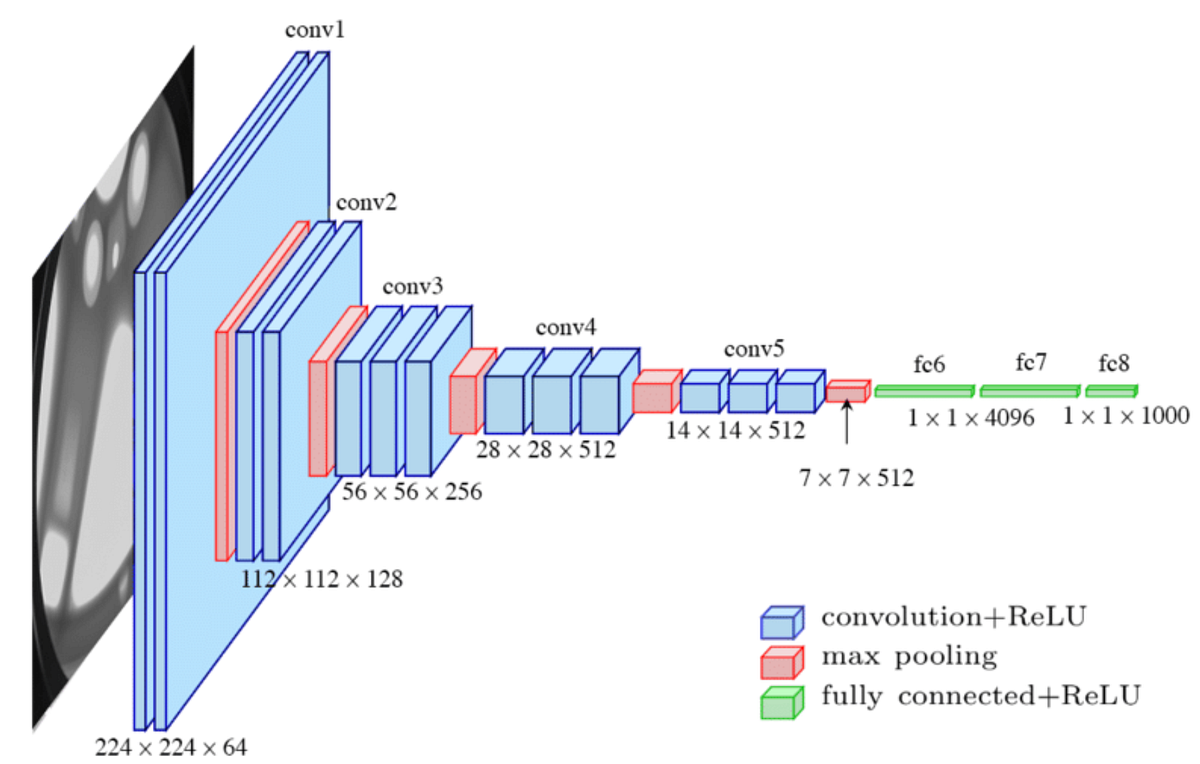
10. Transfer learning con VGG16
En esta sección, usaremos una red VGG16 preentrenada sobre ImageNet y haremos transfer learning para clasificar hojas sanas o enfermas. La idea es:
- Descargar el modelo VGG16 preentrenado usando
torchvision.models. - Congelar las capas convolucionales (el feature extractor) para que no se actualicen sus pesos.
- Reemplazar la parte del clasificador por una capa que se ajuste a nuestra tarea binaria.
- Entrenar solo la parte del clasificador con nuestros datos de hojas, manteniendo los parámetros del feature extractor fijos.
- Utilizar
BCELosspara la pérdida.
Cargamos la VGG
Usamos una arquitectura de este estilo:
# device
device = torch.device("cuda" if torch.cuda.is_available() else "cpu")from torchvision import transforms, models
vgg = models.vgg16(pretrained=True)
# Congelamos las capas convolucionales
for param in vgg.features.parameters():
param.requires_grad = False
# Reemplazamos la última capa del clasificador
# El feature extractor de VGG16 produce un vector de tamaño 25088 a la entrada del clasificador
num_features = 25088
# Creamos un nuevo clasificador
# Mantenemos las dos capas ocultas originales y sólo cambiamos la última
new_classifier = nn.Sequential(
nn.Linear(num_features, 4096),
nn.ReLU(True),
nn.Dropout(p=0.5),
nn.Linear(4096, 1024),
nn.ReLU(True),
nn.Dropout(p=0.5),
nn.Linear(1024, 1) # una salida
)
vgg.classifier = new_classifier
for param in vgg.classifier.parameters():
param.requires_grad = True
vgg.to(device)VGG(
(features): Sequential(
(0): Conv2d(3, 64, kernel_size=(3, 3), stride=(1, 1), padding=(1, 1))
(1): ReLU(inplace=True)
(2): Conv2d(64, 64, kernel_size=(3, 3), stride=(1, 1), padding=(1, 1))
(3): ReLU(inplace=True)
(4): MaxPool2d(kernel_size=2, stride=2, padding=0, dilation=1, ceil_mode=False)
(5): Conv2d(64, 128, kernel_size=(3, 3), stride=(1, 1), padding=(1, 1))
(6): ReLU(inplace=True)
(7): Conv2d(128, 128, kernel_size=(3, 3), stride=(1, 1), padding=(1, 1))
(8): ReLU(inplace=True)
(9): MaxPool2d(kernel_size=2, stride=2, padding=0, dilation=1, ceil_mode=False)
(10): Conv2d(128, 256, kernel_size=(3, 3), stride=(1, 1), padding=(1, 1))
(11): ReLU(inplace=True)
(12): Conv2d(256, 256, kernel_size=(3, 3), stride=(1, 1), padding=(1, 1))
(13): ReLU(inplace=True)
(14): Conv2d(256, 256, kernel_size=(3, 3), stride=(1, 1), padding=(1, 1))
(15): ReLU(inplace=True)
(16): MaxPool2d(kernel_size=2, stride=2, padding=0, dilation=1, ceil_mode=False)
(17): Conv2d(256, 512, kernel_size=(3, 3), stride=(1, 1), padding=(1, 1))
(18): ReLU(inplace=True)
(19): Conv2d(512, 512, kernel_size=(3, 3), stride=(1, 1), padding=(1, 1))
(20): ReLU(inplace=True)
(21): Conv2d(512, 512, kernel_size=(3, 3), stride=(1, 1), padding=(1, 1))
(22): ReLU(inplace=True)
(23): MaxPool2d(kernel_size=2, stride=2, padding=0, dilation=1, ceil_mode=False)
(24): Conv2d(512, 512, kernel_size=(3, 3), stride=(1, 1), padding=(1, 1))
(25): ReLU(inplace=True)
(26): Conv2d(512, 512, kernel_size=(3, 3), stride=(1, 1), padding=(1, 1))
(27): ReLU(inplace=True)
(28): Conv2d(512, 512, kernel_size=(3, 3), stride=(1, 1), padding=(1, 1))
(29): ReLU(inplace=True)
(30): MaxPool2d(kernel_size=2, stride=2, padding=0, dilation=1, ceil_mode=False)
)
(avgpool): AdaptiveAvgPool2d(output_size=(7, 7))
(classifier): Sequential(
(0): Linear(in_features=25088, out_features=4096, bias=True)
(1): ReLU(inplace=True)
(2): Dropout(p=0.5, inplace=False)
(3): Linear(in_features=4096, out_features=1024, bias=True)
(4): ReLU(inplace=True)
(5): Dropout(p=0.5, inplace=False)
(6): Linear(in_features=1024, out_features=1, bias=True)
)
)
class PlantDataset(Dataset):
    def __init__(self, image_paths, labels, img_size=(224,224), mean=None, std=None):
        self.image_paths = image_paths
        self.labels = labels
        self.img_size = img_size
        self.mean = mean
        self.std = std

    def __len__(self):
        return len(self.image_paths)

    def __getitem__(self, idx):
        path = self.image_paths[idx]
        label = self.labels[idx]

        img = Image.open(path).convert("RGB")
        img = img.resize(self.img_size)
        img = np.array(img).astype(np.float32) / 255.0

        # Normalización
        if self.mean is not None and self.std is not None:
            img[...,0] = (img[...,0] - self.mean[0]) / self.std[0]
            img[...,1] = (img[...,1] - self.mean[1]) / self.std[1]
            img[...,2] = (img[...,2] - self.mean[2]) / self.std[2]

        # Transponer a CxHxW
        img = np.transpose(img, (2, 0, 1))
return torch.from_numpy(img), torch.tensor(label, dtype=torch.float32)train_dataset, test_dataset = load_dataset(root)
train_loader = DataLoader(train_dataset, batch_size=64, shuffle=True, num_workers=0)
test_loader = DataLoader(test_dataset, batch_size=64, shuffle=False, num_workers=0)Train size: 3601, Test size: 901
batch_size = 128
epochs = 20
train_losses_vgg = []
test_losses_vgg = []
train_accuracies_vgg = []
test_accuracies_vgg = []

criterion = nn.BCEWithLogitsLoss()
optimizer = optim.Adam(vgg.parameters(), lr=0.001)

for epoch in range(1, epochs+1):
    train_loss = train_one_epoch(vgg, train_loader, optimizer, device, criterion)
    # Evaluamos en train y test con el modelo en modo eval
    train_loss_eval, train_acc_eval = evaluate(vgg, train_loader, device, criterion)
    test_loss_eval, test_acc_eval = evaluate(vgg, test_loader, device, criterion)

    train_losses_vgg.append(train_loss_eval)
    test_losses_vgg.append(test_loss_eval)
    train_accuracies_vgg.append(train_acc_eval)
    test_accuracies_vgg.append(test_acc_eval)

    print(f"Epoch {epoch}: Train Loss: {train_loss:.4f} | Train Acc: {train_acc_eval:.4f} | Test Acc: {test_acc_eval:.4f}")
Epoch 1: Train Loss: 0.6315 | Train Acc: 0.9514 | Test Acc: 0.9290 Epoch 2: Train Loss: 0.1596 | Train Acc: 0.9664 | Test Acc: 0.9156 Epoch 3: Train Loss: 0.1123 | Train Acc: 0.9797 | Test Acc: 0.9267 Epoch 4: Train Loss: 0.0938 | Train Acc: 0.9919 | Test Acc: 0.9412 Epoch 5: Train Loss: 0.0603 | Train Acc: 0.9964 | Test Acc: 0.9401 Epoch 6: Train Loss: 0.0473 | Train Acc: 0.9939 | Test Acc: 0.9345 Epoch 7: Train Loss: 0.0484 | Train Acc: 0.9881 | Test Acc: 0.9212 Epoch 8: Train Loss: 0.0191 | Train Acc: 0.9989 | Test Acc: 0.9345 Epoch 9: Train Loss: 0.0356 | Train Acc: 0.9964 | Test Acc: 0.9301 Epoch 10: Train Loss: 0.0289 | Train Acc: 0.9981 | Test Acc: 0.9478 Epoch 11: Train Loss: 0.0258 | Train Acc: 0.9997 | Test Acc: 0.9456 Epoch 12: Train Loss: 0.0096 | Train Acc: 0.9994 | Test Acc: 0.9467 Epoch 13: Train Loss: 0.0121 | Train Acc: 0.9994 | Test Acc: 0.9323 Epoch 14: Train Loss: 0.0258 | Train Acc: 0.9961 | Test Acc: 0.9301 Epoch 15: Train Loss: 0.0341 | Train Acc: 0.9958 | Test Acc: 0.9267 Epoch 16: Train Loss: 0.0187 | Train Acc: 1.0000 | Test Acc: 0.9412 Epoch 17: Train Loss: 0.0169 | Train Acc: 1.0000 | Test Acc: 0.9401 Epoch 18: Train Loss: 0.0328 | Train Acc: 0.9997 | Test Acc: 0.9367 Epoch 19: Train Loss: 0.0214 | Train Acc: 1.0000 | Test Acc: 0.9412 Epoch 20: Train Loss: 0.0159 | Train Acc: 0.9992 | Test Acc: 0.9412
# Pintar curvas
plot_curves(train_losses_vgg, test_losses_vgg, train_accuracies_vgg, test_accuracies_vgg)
# Predecir en test para matriz de confusión
vgg.eval()
all_preds = []
all_labels = []

with torch.no_grad():
    for images, labels in test_loader_aug:
        images = images.to(device)
        labels = labels.to(device)
        outputs = vgg(images)
        preds = (outputs.view(-1) >= 0.5).long()
        all_preds.append(preds.cpu().numpy())
        all_labels.append(labels.cpu().numpy())

all_preds = np.concatenate(all_preds)
all_labels = np.concatenate(all_labels)

# Pintar matriz de confusión
plot_confusion_matrix(all_labels, all_preds, classes=['Sana', 'Enferma'])

# Calcular tasa de falsos positivos
from sklearn.metrics import confusion_matrix

cm = confusion_matrix(all_labels, all_preds)
tn, fp, fn, tp = cm.ravel()
fpr = fp / (fp + tn) if (fp + tn) > 0 else 0